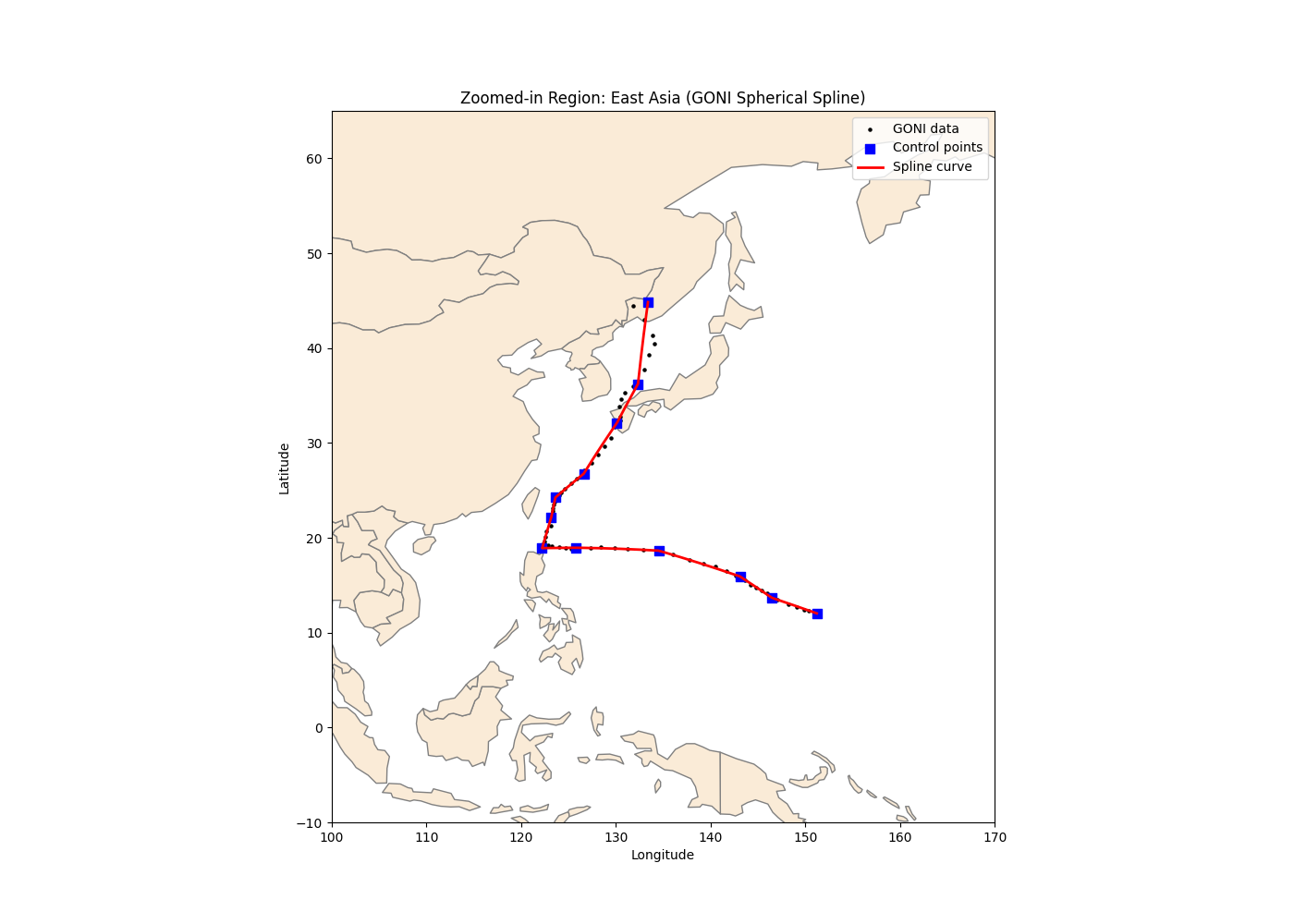
GONI Example

This example demonstrates fitting a penalized spherical spline to the GONI dataset and plotting the resulting spline curve on a world map.

Best λ index: 5
Control points (cartesian):
[[-0.85719402  0.47093044  0.20842968]
 [-0.81024223  0.5363929   0.23619944]
 [-0.76899269  0.57738131  0.27437396]
 [-0.664392    0.67557648  0.31965557]
 [-0.55299875  0.76729572  0.32473013]
 [-0.5044202   0.80037947  0.32396444]
 [-0.50697264  0.77541588  0.3764425 ]
 [-0.50487473  0.75924853  0.41066187]
 [-0.53257145  0.71676055  0.45013549]
 [-0.54586299  0.64801127  0.53114498]
 [-0.54360735  0.59660668  0.59038253]
 [-0.48712871  0.51516339  0.70520373]]

# ----------------------------------------------------
# Imports
# ----------------------------------------------------
import numpy as np
import pandas as pd
import matplotlib.pyplot as plt
import geopandas as gpd

import spheresmooth as ss
from spheresmooth.loads import load_world_map


# ----------------------------------------------------
# 1. Load GONI spherical data (t, theta, phi)
# ----------------------------------------------------
goni = ss.load_goni()   # DataFrame: [t, theta, phi]

t = goni.iloc[:, 0].values
spherical = goni.iloc[:, 1:3].values   # (theta, phi)


# ----------------------------------------------------
# 2. Spherical → Cartesian
# ----------------------------------------------------
goni_cartesian = ss.spherical_to_cartesian(spherical)


# ----------------------------------------------------
# 3. Quantile knots + lambda sequence
# ----------------------------------------------------
dimension = 12     # moderate for quick Sphinx-Gallery execution
initial_knots = ss.knots_quantile(t, dimension)

lambda_seq = np.exp(np.linspace(np.log(1e-6), np.log(1), 25))


# ----------------------------------------------------
# 4. Penalized spherical spline fit
# ----------------------------------------------------
fit = ss.penalized_linear_spherical_spline(
    t=t,
    y=goni_cartesian,
    dimension=dimension,
    initial_knots=initial_knots,
    lambdas=lambda_seq
)

bic_list = fit["bic_list"]
fits = fit["fits"]

best_index = np.argmin(bic_list)
best_fit = fits[best_index]
control_points = best_fit["control_points"]
knots = best_fit["knots"]

print("Best λ index:", best_index)
print("Control points (cartesian):")
print(control_points)


# ----------------------------------------------------
# 5. Convert control points to latitude/longitude
# ----------------------------------------------------
cp_spherical = ss.cartesian_to_spherical(control_points)
cp_deg = np.degrees(cp_spherical)

cp_df = pd.DataFrame({
    "latitude": 90 - cp_deg[:, 0],
    "longitude": cp_deg[:, 1],
})


# ----------------------------------------------------
# 6. Evaluate piecewise geodesic curve
# ----------------------------------------------------
ts = np.linspace(0, 1, 2000)

curve_cart = ss.piecewise_geodesic(ts, control_points, knots)
curve_sph = ss.cartesian_to_spherical(curve_cart)
curve_deg = np.degrees(curve_sph)

curve_df = pd.DataFrame({
    "latitude": 90 - curve_deg[:, 0],
    "longitude": curve_deg[:, 1],
})


# ----------------------------------------------------
# 7. Original GONI data → (lat, lon)
# ----------------------------------------------------
goni_deg = np.degrees(spherical)

goni_df = pd.DataFrame({
    "latitude": 90 - goni_deg[:, 0],
    "longitude": goni_deg[:, 1],
})


# ----------------------------------------------------
# 8. Figure: World map + GONI + fitted curve (single figure)
# ----------------------------------------------------
import geopandas as gpd
import matplotlib.pyplot as plt

# Load world shapefile
world_path = load_world_map()
world = gpd.read_file(world_path)

fig, ax = plt.subplots(figsize=(14, 10))

# World map
world.plot(ax=ax, color="antiquewhite", edgecolor="gray")

# Raw GONI data
ax.scatter(
    goni_df["longitude"], goni_df["latitude"],
    s=5, color="black", label="GONI data"
)

# Control points
ax.scatter(
    cp_df["longitude"], cp_df["latitude"],
    s=60, color="blue", marker="s", label="Control points"
)

# Fitted spline curve
ax.plot(
    curve_df["longitude"], curve_df["latitude"],
    color="red", linewidth=2, label="Spline curve"
)

# Zoom bounds (East Asia)
ax.set_xlim(100, 170)
ax.set_ylim(-10, 65)

ax.set_xlabel("Longitude")
ax.set_ylabel("Latitude")
ax.set_title("Zoomed-in Region: East Asia (GONI Spherical Spline)")
ax.legend()

plt.show()