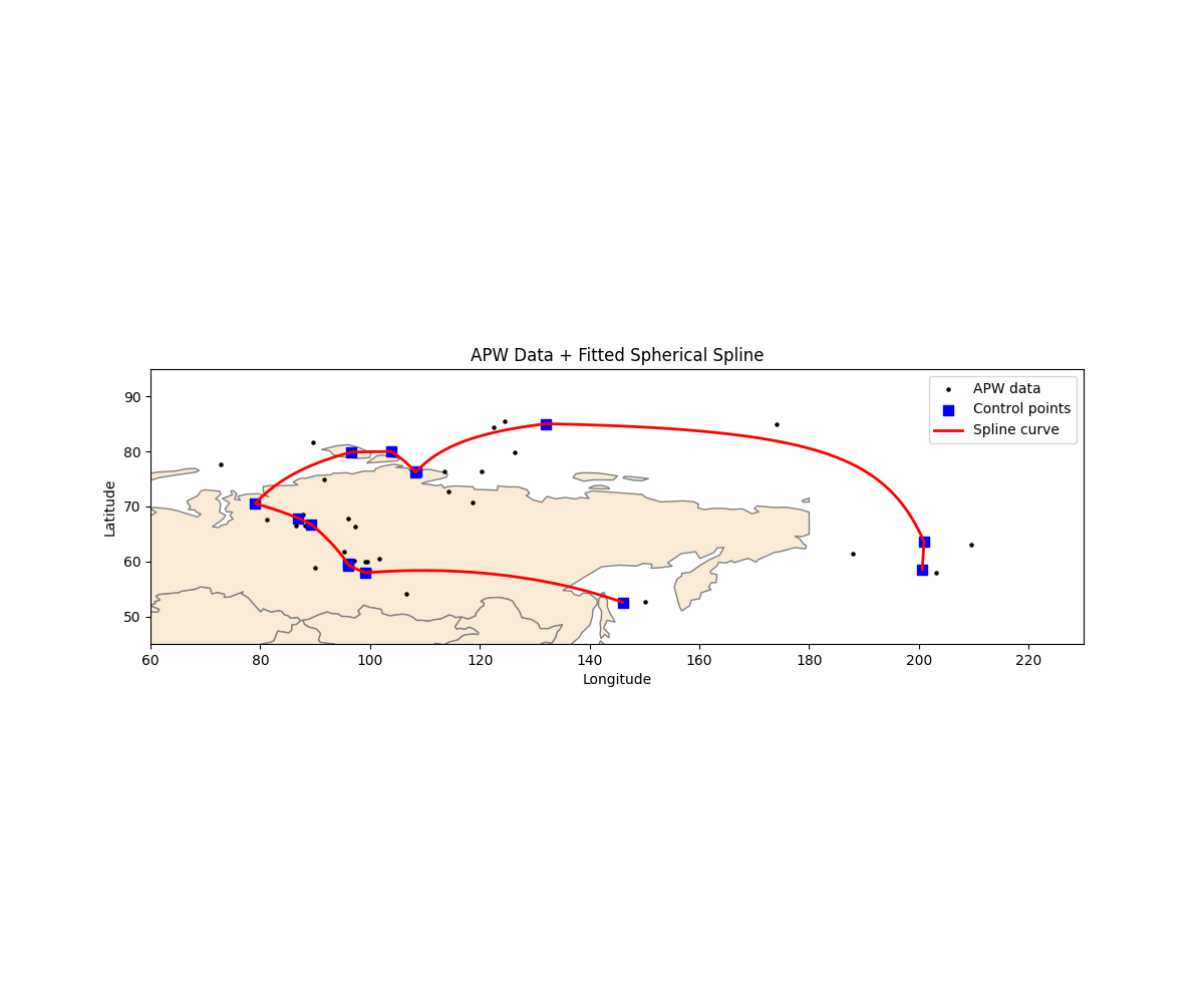
APW Example

This example demonstrates fitting a penalized spherical spline to the Apparent Polar Wander (APW) path and plotting the result on a world map.

Best λ index: 28
Control points (cartesian):
[[-0.48799339 -0.18359966  0.85331918]
 [-0.41541484 -0.15888491  0.89564842]
 [-0.05778102  0.06411578  0.9962683 ]
 [-0.07458957  0.22358783  0.97182554]
 [-0.07418727  0.22529426  0.97146217]
 [-0.0415261   0.16843219  0.98483815]
 [-0.02021256  0.17445605  0.98445748]
 [ 0.06310967  0.32686588  0.94296122]
 [ 0.02050204  0.37587383  0.92644403]
 [ 0.00531943  0.39425323  0.91898645]
 [-0.05242935  0.50251786  0.86297564]
 [-0.05414767  0.50781569  0.85976232]
 [-0.08338042  0.52447341  0.84733426]
 [-0.50457063  0.33962265  0.7937663 ]]

# ----------------------------------------------------
# Imports
# ----------------------------------------------------
import numpy as np
import pandas as pd
import matplotlib.pyplot as plt
import geopandas as gpd

import spheresmooth as ss
from spheresmooth.loads import load_world_map


# ----------------------------------------------------
# 1. Load APW spherical data (θ, φ in radians)
# ----------------------------------------------------
apw = ss.load_apw()   # pandas DataFrame: [t, theta, phi]

t = apw.iloc[:, 0].values
spherical = apw.iloc[:, 1:3].values   # (theta, phi)


# ----------------------------------------------------
# 2. Spherical → Cartesian
# ----------------------------------------------------
apw_cartesian = ss.spherical_to_cartesian(spherical)


# ----------------------------------------------------
# 3. Quantile knots
# ----------------------------------------------------
dimension = 15
initial_knots = ss.knots_quantile(t, dimension)

lambda_seq = np.exp(np.linspace(np.log(1e-7), np.log(1), 40))


# ----------------------------------------------------
# 4. Penalized spherical spline fit
# ----------------------------------------------------
fit = ss.penalized_linear_spherical_spline(
    t=t,
    y=apw_cartesian,
    dimension=dimension,
    initial_knots=initial_knots,
    lambdas=lambda_seq
)

bic_list = fit["bic_list"]
fits = fit["fits"]

best_index = np.argmin(bic_list)
best_fit = fits[best_index]
control_points = best_fit["control_points"]
knots = best_fit["knots"]

print("Best λ index:", best_index)
print("Control points (cartesian):")
print(control_points)


# ----------------------------------------------------
# 5. Convert control points → (theta, phi)
# ----------------------------------------------------
cp_spherical = ss.cartesian_to_spherical(control_points)
cp_deg = np.degrees(cp_spherical)

cp_df = pd.DataFrame({
    "latitude": 90 - cp_deg[:, 0],
    "longitude": cp_deg[:, 1]
})


# ----------------------------------------------------
# 6. Evaluate piecewise geodesic curve
# ----------------------------------------------------
ts = np.linspace(0, 1, 2000)

curve_cart = ss.piecewise_geodesic(ts, control_points, knots)
curve_sph = ss.cartesian_to_spherical(curve_cart)
curve_deg = np.degrees(curve_sph)

curve_df = pd.DataFrame({
    "latitude": 90 - curve_deg[:, 0],
    "longitude": curve_deg[:, 1]
})


# ----------------------------------------------------
# 7. Original APW data → (lat, lon)
# ----------------------------------------------------
apw_deg = np.degrees(spherical)

apw_df = pd.DataFrame({
    "latitude": 90 - apw_deg[:, 0],
    "longitude": apw_deg[:, 1]
})


# ----------------------------------------------------
# 8. Plot world map + APW + spline curve (single figure)
# ----------------------------------------------------
fig, ax = plt.subplots(figsize=(12, 10))

# World map
world_path = load_world_map()
world = gpd.read_file(world_path)
world.plot(ax=ax, color="antiquewhite", edgecolor="grey")

# Raw APW data
ax.scatter(
    apw_df["longitude"], apw_df["latitude"],
    s=5, color="black", label="APW data"
)

# Control points
ax.scatter(
    cp_df["longitude"], cp_df["latitude"],
    s=60, color="blue", marker="s", label="Control points"
)

# Fitted spline curve
ax.plot(
    curve_df["longitude"], curve_df["latitude"],
    c="red", linewidth=2, label="Spline curve"
)

# ---------------------------
# Zoom region
# ---------------------------
ax.set_xlim(60, 230)
ax.set_ylim(45, 95)

ax.set_xlabel("Longitude")
ax.set_ylabel("Latitude")
ax.set_title("APW Data + Fitted Spherical Spline")
ax.legend()

plt.show()